1. Introduction
\[r = g(f, \theta).\]General reward function을 추정하는 이전의 접근들은 대체로 hand selected features에 대한 weighted linear function를 reward function으로 정의하는 방법을 사용하였다. 이후 linear model에 대한 한계점에 의해 여러가지 non-parametric methods (가령 Gaussian Process 등)가 대안책으로 제시되었지만, kernel machine의 사용에 의해 학습에 많은 데이터를 필요로 하거나 experiences state-rewards pairs의 수에 따라 query의 time complexity가 증가하는 등 그 나름의 문제점을 갖고 있었다.
Linear Model
\[g(f, \theta) = \theta^T f.\]Linear Model with Feature Compositio=
\[g(f, \theta, \Phi) = \theta^T \Phi(f).\]Here \(\Phi\) denotes a set of composite features which are jointly learned as part of the objective function.
Gaussian Processes IRL
\[g(f, \theta, \chi_\mu, \mu) = K_{f, \mu}^T K_{\mu, \mu}^{-1} \mu.\]\(K_{f, \mu}\) denotes the covariance of the reward at \(f\) with the active set reward values \(\mu\) located at \(X_\mu\) and \(K_{\mu, \mu}\) denotes the covariance matrix of the rewards in the active set computed via a covariance matrix of the rewards in the active set computed via a covariance function \(k_\theta (f_i, f_j)\) with hyperparameters \(\theta\).
본 연구에서는 convolution 연산을 통해 (gridded representation인) raw input에 대한 별도의 전처리 없이도 end-to-end learning을 가능하게 하는 방법을 제시한다. Neural network (이하 NN)가 비젼, 자연어처리, 음성인식 등 다양한 분야에서 아주 좋은 성능을 발휘함은 이미 검증된 바가 있으며, layered structure 내에서 사용되는 수많은 nonlinearity가 조합 및 재사용을 통해 compact representation을 도출한다고 알려져있다. 또한 NN은 test time에서 주어진 demonstration 갯수에 상관없이 상수 계산복잡도(\(O(1)\))로 결과를 출력한다는 점도 큰 장점이다.
Maximum Entropy Deep Inverse Reinforcement Learning의 주된 기여는 IRL에 대한 Maximum Entropy paradigm을 기본으로 deep architecture에 대한 훈련을 통해 입력에 대한 전처리작업(manually crafted feature design) 없이도 현존하는 다른 SOTA methods와 비교해 나쁘지 않은 성능을 보인다는 점이다.
2. Training Procedure
IRL 문제를 푸는 것은 주어진 reward structure와 parameter \(\theta\)에 대해 observing expert demonstrations, \(D\),를 MAP하는 것이라 볼 수 있다.
\[\begin{align} L(\theta) &= \log P(D, \theta \mid r) = \log P(D \mid r) + \log P(\theta).\\ L_D &= \log P(D \mid r)\\ L_\theta &= \log P(\theta) \end{align}\]Note: \(\log P(D, \theta \mid r) = \log P(D \mid r) + \log P(\theta)\)가 성립하는 이유?
Guess)
\[\log P(D, \theta \mid r) = \log P(D \mid r) + log P(\theta \mid r)\]이때 \(\log P(\theta \mid r)\)를 MAP관점에서 likelihood * prior로 보면 이는,
\[\log P(r \mid \theta)*P(\theta) = \log P(r \mid \theta) + \log P(\theta).\]고정된 \(\theta\)에 대해 일정한 reward function, \(r\),을 보장하므로 \(\log P(r \mid \theta) = 0\).
즉, \(\log P(\theta \mid r) = \log P(\theta)\).
3. Gradient Term
Gradient Term은 다음과 같이 model parameter \(\theta\)에 대한 data term과 model regulariser (weight decay) term으로 나누어 볼 수 있다.
\[\frac{\partial L}{\partial \theta} = \frac{\partial L_D}{\partial \theta} + \frac{\partial L_\theta}{\partial \theta}.\]이 중 data term에 대해 chain rule을 적용해보자. (차후 알고리즘에서는 model regulariser term에 대해서는 명시적으로 다루지 않는다.)
\[\begin{align} \frac{\partial L_D}{\partial \theta} &= \frac{\partial L_D}{\partial r} \cdot \frac{\partial r}{\partial \theta}\\ &= (\mu_D - \mathbb{E}[\mu]) \cdot \frac{\partial}{\partial \theta} g(f, \theta),\\ \text{where } r &= g(f, \theta). \end{align}\]위의 \(\mu_D - \mathbb{E}[\mu]\)는 아래 최종 유도된 \(\nabla_\psi L\)의 공식에서 \(\nabla_\psi r_\psi = 1\)로 둔 것과 같다. (r에 대한 미분이므로)
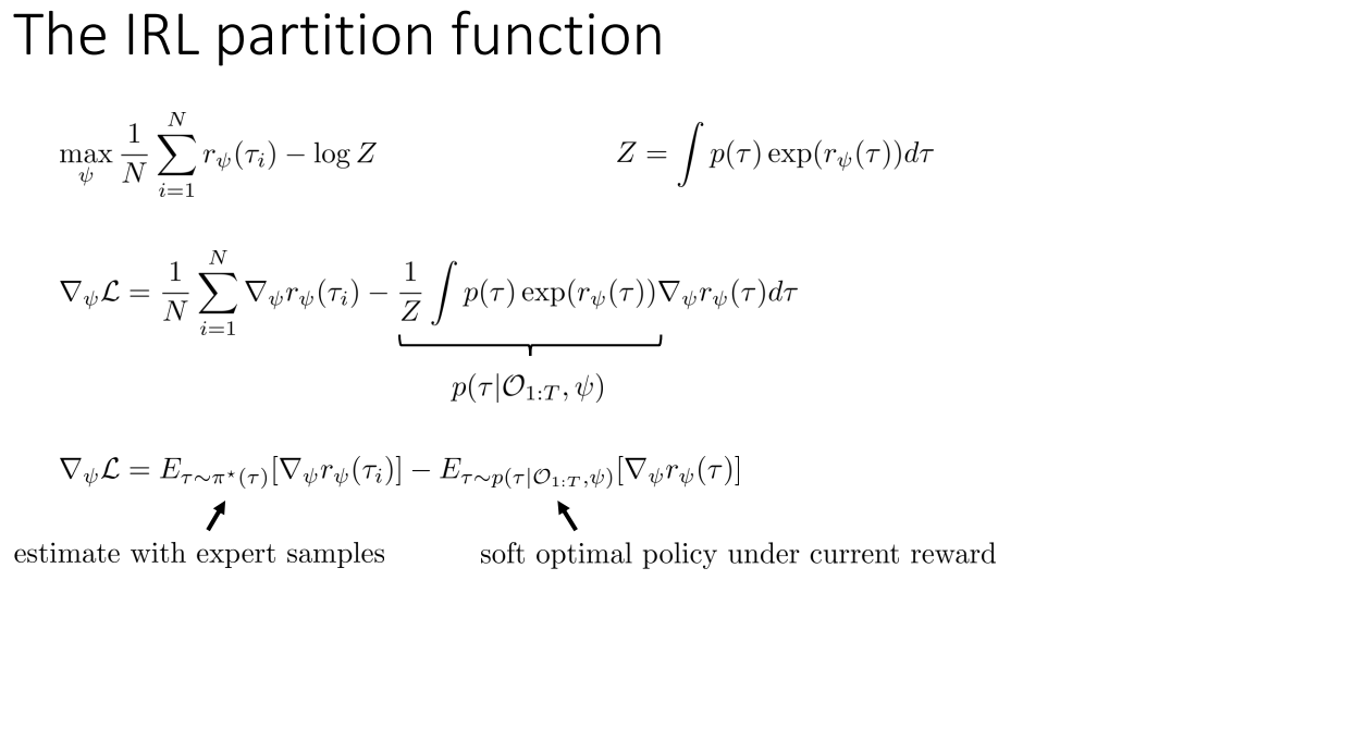
즉,
\(\mathbb{E}[\mu] = \sum_{\zeta: \{s, a\} \in \zeta} P(\zeta | r)\) \(\mu_D = \sum_{a=1}^{A} \mu_D^a, \text{where } \mu_D^a \text{ is the expert's state action frequency.}\)
4. Algorithms
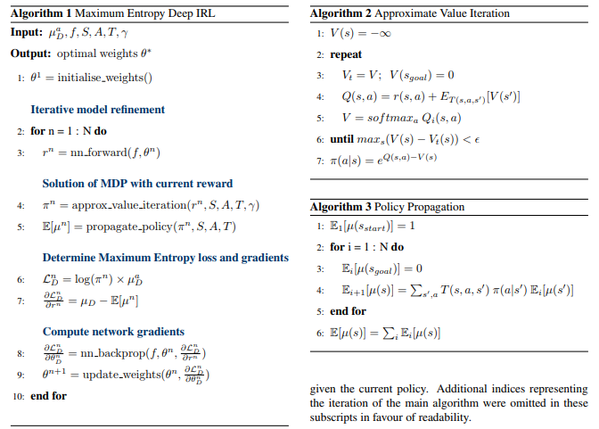
Guess) Algorithm1의 line 6는 log policy와 state action frequency의 곱이므로 minus entropy로 보여진다. 이를 최소화해야 maximum entropy의 효과가 발생하는 것일텐데, line 7을 점차 0이되게 함으로써 entropy를 최대화한다는 의도인 것 같다. (line6는 concave 함수에 대한 nonnegative linear combination이므로 concave 함수 -도메인이 convex set이라 가정)
5. Experiment Results
학습에 좀 더 많은 데이터를 요구하긴 하지만, demonstration sample의 갯수에 상관없이 일정한 algorithmic complexity를 보이면서 SOTA 방식들에 비교해 나쁘지 않은 성능을 보인다. 이러한 특성에 의거해 life-long learning scenario에 사용되기 적합한 알고리즘일 것이다.