1. Introduction
실전에서 잘 동작하는 cost function을 정의하는 것에는 항상 어려움이 따른다. 주로 다음과 같은 이유에서다.
- 유용한 형태의 feature를 설계하는 것
- Iterative cost optimization의 inner loop에서 현재 cost에 대한 최적의 policy를 찾는 연산 (complexity issue)
본 연구에서는 이에 대한 해법으로 neural network를 사용한 nonlinear function approximation과 2가지 regularization techniques (for general purpose and for episodic domain)를 제안하다.
또한 이전 연구(Ziebart et al., 2008)에서 cost learning의 inner loop에서 policy search를 했던 것과 달리, Guided Cost Learning에서는 policy search의 inner loop에서 cost에 대한 업데이트를 한다. 즉, policy optimization이 cost function을 점차 더 좋은 형태로 ‘가이드’하는 방식이다.
몇 가지 simulated benchmark tasks에서 guided cost learning은 이전 방식들과 비교에 훨씬 좋은 성능을 보여준다.
2. Preliminaries and Overview
The probabilistic maximum entropy inverse optimal control framework (Ziebart et al., 2008)의 아이디어를 기초로 한다. 여기서 expert는 다음의 분포에서 suboptimal trajectories \({\tau_i}\)를 추출(sample)하는 것으로 가정한다. \(p(\tau) = \frac{1}{Z} \exp(-c_\theta (\tau))\)
문제는 partition function Z를 계산하는 것이 굉장히 어렵다는 것이다. Small, discrete domain이라면 dynamic programming을 사용하여 Z의 계산이 가능하지만, large/continuous space라면 이런 방법으로는 Z의 계산이 불가능해진다. 이 연구에서는 sample-based approach를 통해 partition function Z를 계산한다. 이 방식은 unknown system dynamics에 대해서도 inverse optimal control을 시행할 수 있게한다.
IOC / IRL 방법론에서는 보편적으로 cost function \(c_\theta (x_t, u_t)\)를 hand-crafted feature와 parameter 간의 linear combination으로 정의한다. 하지만 이러한 정의는 더욱 복잡한 도메인에서 적용하기에는 한계가 있으므로 \(c_\theta (x_t, u_t)\)를 raw sensory input에 대한 neural network로 정의한다.
3. Guided Cost Learning
이 method의 중심에 있는 아이디어는 cost distribution \(p(\tau) = \frac{1}{Z} \exp(-c_\theta (\tau))\)의 maximum entropy에 맞추어가는 방향으로 sampling distribution을 조정해가는 것이다. Phicycal system에서 생성된 sample은 policy를 향상시키고 partition function을 좀 더 잘 추정하기 위해 사용한다.
Sample-based approximation 방식의 IOC objective (\(L_{IOC}\))를 유도해보자. \(L_{IOC}\)는 \(p(\tau) = \frac{1}{Z} \exp(-c_\theta (\tau))\)에 대한 negative log-likelihood로부터 시작한다.
\[L_{IOC} = \frac{1}{N} \sum_{\tau_i \in D_{demo}} c_\theta(\tau_i) + \log Z\]- \(D_{demo}\): \(N\)개의 demonstrated trajectories
- \(D_{sample}\): \(M\)개의 background samples
- \(q\): trajectories \(\tau_j\)를 추츨하는 background distribution (policy)
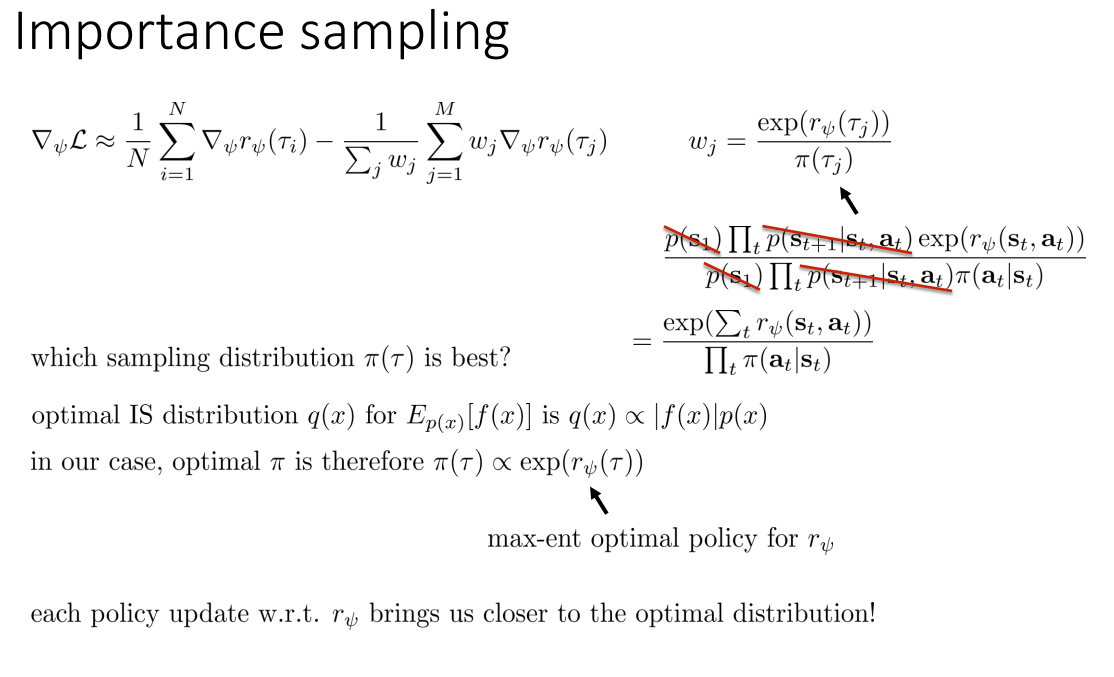
- \(w_j = \frac{\exp(-c_\theta (\tau_j))}{q(\tau_j)}\) (importance sampling)
- \(Z = \sum_j w_j\)
\(L_{IOC}\)의 \(\theta\)에 대한 gradient는 다음과 같다.
\[\frac{d L_{IOC}}{d \theta} = \frac{1}{N} \sum_{\tau_i \in D_{demo}} \frac{d c_{\theta}}{d \theta} (\tau_i) - \frac{1}{Z} \sum_{\tau_j \in D_{samp}} w_j \frac{d c_\theta}{d \theta} (\tau_j)\]여기서 사용된 importance sampling에 대해서는 cs294 lec16: Inverse Reinforcement Learning에서 좀 더 자세히 다루고 있다.
4. Algorithms
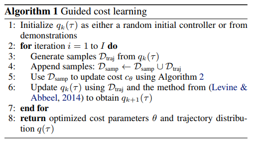
Background distribution \(q(\tau)\)는 Gaussian으로 정의한다. 또한 현재의 cost function \(c_\theta (\tau)\)에 대해 modified LQR backward pass를 통해 \(q(\tau)\)를 adaptively refine한다. 매 policy optimization procedure에서는 KL-divergence constraint (\(D_{KL}(q(\tau) \| \hat{q}(\tau)) \le \epsilon\))를 이용한 trust region method로 poor initial cost estimation에 대해 overffiting하는 것을 예방한다.
추가로 위 알고리즘에 약간의 수정을 더하여 maximum entropy version의 objective로 재정의 할 수 있다.
\[\min_q E_q[c_\theta (\tau)] - \mathcal{H}(\tau)\]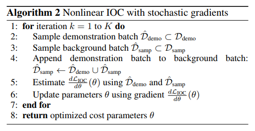
실제로 알고리즘을 시행하다보면 objective가 unbounded하는 이슈가 발생하곤 하는데, 알고리즘 line 4에서처럼 sampled demonstraion을 background sample에 추가하는 것으로 이를 완화시킬 수 있다.
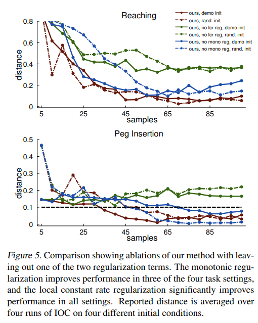
5. Regularization
일반적으로 사용하는 \(\theta\)에 대한 \(l_1\), \(l_2\) penalty는 때때로 high-dimensional nonlinear const function에 대해 잘 동작하지 않는 경우가 발생한다. 각 entry는 parameter vector에 의해 각각 cost에 상당히 다른 영향을 미치기 때문이다. 이에 두 가지 새로운 regularizer를 소개한다.
a. Locally at a constant rate (lcr)
\[g_{lcr}(\tau) = \sum_{x_t \in \tau} [(c_\theta (x_{t+1}) - c_\theta (x_t)) - (c_\theta (x_t) - c_\theta (x_{t-1}))]^2\]위는 high-frequency variation을 낮춰주는 term이다. 이는 overfitting을 줄여주는 역할을 한다. 실험을 통해 대체로 slow-changing cost가 잘 작동함을 보였다.
b. Monotonically decrease cost (mono)
\[g_{mono}(\tau) = \sum_{x_t \in \tau} [\max(0, c_\theta (x_t) - c_\theta (x_{t-1}) - 1)]^2\]Squared hinge loss에 의해 demo trajectory의 cost를 strictly monotonically 줄여준다. Demonstration이 (potentially nonlinear) manifold에서 goal에 대해 monotonic progress를 발생시킨다고 가정하였다.
두 regularizer에 대한 실험결과는 다음과 같다.
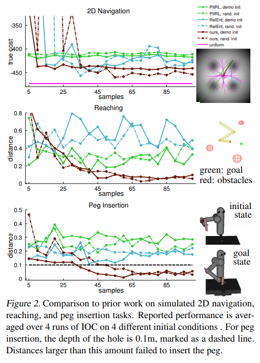
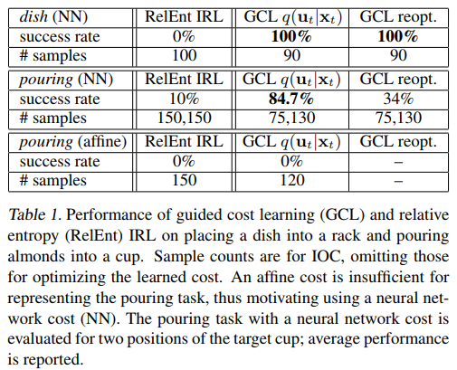
6. Experimental Results
Mujoco simulator (2D navigation, 3-link arm reacher, 3D peg insertion)와 real-world tasks (dish placement, pouring)에 대해 실험한 결과다. 각각 20~32개, 25~30개의 human demonstration을 사용했다.