1. Introduction
본 논문에서는 서로 다른 세가지 도메인에서의 아이디어(MaxEnt IRL, GAN, EBM)가 다음 사실들을 통해 서로 깊은 연관성이 있음을 보일것이다.
- Generator의 density를 구할 수 있는 경우(can be efficiently evaluated), GAN이 sample-based MaxEnt IRL과 수학적으로 동일함
- IRL의 maximum entropy formulation이 energy-based model (EBM)의 특수한 형태 (special case)임
- GAN의 특정 형태 (particular form)가 EBM을 학습 시키기 위해 사용될 수 있음
2. Background
GAN, EBM, IRL에 대해 간략히 설명한다.
2.1 Generative Adversarial Networks
다음 두 가지 모델을 동시에 학습시키는 방법이다.
- Discriminator: 입력이 data distribution \(p(x)\)를 따르는 actual sample인지 혹은 generator로부터의 출력인지 구분
- Generator: noise를 입력으로 하여 actual sample과 유사한 sample을 생성
2.2 Energy-Based Model
Sample \(x\)에 대한 energy value \(E_\theta (x)\)로 이루어져 있으며, Boltzmann distribution으로 data를 모델링한다. High-dimensional problem에서 partition function \(Z\)를 계산하는 것은 보통 intractable한 문제로 알려져있다.
\[p_\theta (x) = \frac{1}{Z} \exp(-E_\theta(x))\]2.3 Inverse Reinforcement Learning
Maximum entropy inverse reinforcement learrning은 demonstration을 다음과 같은 Boltzmann distribution으로 모델링한다. (여기서 energy는 cost function \(c_\theta\)로 정의한다.) \(p_\theta (\tau) = \frac{1}{Z} \exp (-c_\theta (\tau))\) 이때, \(\tau = \{x_1,u_1, ..., x_T,u_T\}\)는 trajectory이고, \(c_\theta(\tau) = \sum_t c_\theta(x_t, u_t)\)는 \(\theta\)로 parameterized된 학습된 cost function이다. 또한 partition function \(Z\)는 \(\int p(\tau)\exp(-c_\theta (\tau)) d\tau\)이다. (중요: 아래의 유도과정에서 environment dynamics \(p(\tau)\)는 deterministic function이라 가정한다.)
Parameter \(\theta\)는 demonstration에 대한 MLE로 계산되며, 여기서도 마찬가지로 large or continuous domain에서 partition function을 추정하는 것은 계산적인 주요 도전과제에 해당한다.
Guided Cost Learning에서는 MaxEnt IRL formulation에서 iterative sample-based 방식으로 \(Z\)를 추정하였다. 좀 더 자세히 말하자면 다음과 같이 sampling distribution \(q(\tau)\)와 importance sampling을 이용하여 \(Z\)를 추정한다.
\[\begin{align*} L_{cost} &= \mathbb{E}_{\tau \sim p} [-\log p_\theta(\tau)] = \mathbb{E}_{\tau \sim p} [c_\theta(\tau)] + \log Z\\ &= \mathbb{E}_{\tau \sim p} [c_\theta (\tau)] + \log \big( \mathbb{E}_{\tau \sim q} \big[ \frac{\exp(-c_\theta(\tau))}{q(\tau)} \big] \big). \end{align*}\](Note: \(p\)가 stochastic function이라면 2번째 term의 \(\exp\) 앞에 \(p\)가 곱해져야 할 것이다.)
헌데, 이러한 importance sampling 방식은 sampling distribution \(q\)가 높은 \(\exp(-c_\theta (\tau))\) 값을 가진 trajectory를 잘 커버하지 못하는 경우 high variance 문제를 야기할 수 있다. 이 문제(coverage problem)를 완화하기 위해 demonstration data distribution과 generated sample distribution을 혼합한 mixture distribution을 사용한다: \(\mu = \frac{1}{2}p + \frac{1}{2}q\). 이때 demonstration data distribution을 근사하는 분포 \(\tilde{p}\)를 사용한 mixture distribution이 \(\tilde{\mu} = \frac{1}{2}\tilde{p} + \frac{1}{2}q\)라 하면, guided cost learning은 다음과 같이 변형된다.
\[L_{cost} = \mathbb{E}_{\tau \sim p} [c_\theta (\tau)] + \log \big( \mathbb{E}_{\tau \sim \mu} \big[ \frac{\exp(-c_\theta(\tau))}{\frac{1}{2}\tilde{p} + \frac{1}{2}q} \big] \big).\]Guided cost learning의 학습 과정은 \(q\)와 \(\frac{1}{Z}\exp(-c_\theta(\tau))\)의 KL divergence를 최소화시키는 것과도 같다.
\[\begin{align*} L_{sampler} &= \mathbb{E}_{\tau \sim q}[log \frac{q(\tau)}{\frac{1}{Z}\exp(-c_\theta(\tau))}]\\ &= \mathbb{E}_{\tau \sim q} [c_\theta(\tau)] + \mathbb{E}_{\tau \sim q} [\log q(\tau)] + \log Z \end{align*}\]3. GANs and IRL
Discriminator가 특정형태로 정의되어 있을때, GAN의 discriminator가 learned cost를 내포하며 또한 generator가 policy를 나타냄을 알아보겠다.
우선 optimal discriminator의 형태부터 살펴보자. (from GAN)
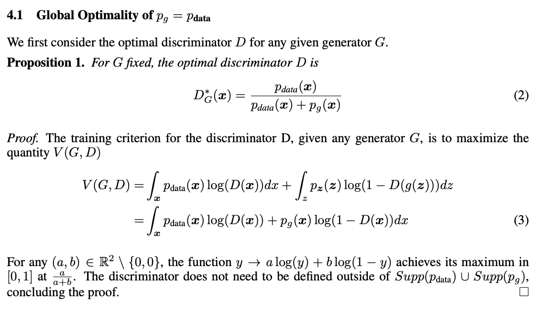
Fixed genetator density를 \(q(\tau)\), data의 actual distribution을 \(p(\tau)\)라 한다면 위의 optimal discriminator는 아래와 같이 다시 쓸 수 있다.
\[D^* (\tau) = \frac{p(\tau)}{p(\tau) + q(\tau)}\]Traditional GAN algorithm에서 discriminator는 위 값을 곧바로 출력할 수 있게끔 학습된다. 여기서 \(D\)를 바로 추정하는 것이 아니라 parameterized \(p\)를 통해 추정한다고 해보자.
\[D_\theta (\tau) = \frac{p_\theta(\tau)}{p_\theta(\tau) + q(\tau)}\]MaxEnt IRL과의 연결성을 만들기 위해 estimated data density를 Boltzmann distribution으로 바꿔보겠다.
\[D_\theta (\tau) = \frac{\frac{1}{Z}\exp(-c_\theta(\tau))}{\frac{1}{Z}\exp(-c_\theta(\tau)) + q(\tau)}\]\(\frac{1}{Z}\exp(-c_\theta(\tau)) = p(\tau)\)를 만족할때 \(D_\theta (\tau) = D^*(\tau)\)가 성립할 것이다.
그럼 이제 discriminator의 loss에 위 \(D_\theta\)를 대입해보고, 이것을 maximum entropy IRL의 log-likelihood objective와 비교해보도록 하겠다.
Discriminator’s loss
\[\begin{align*} L_{discriminator}(D_\theta) &= \mathbb{E}_{\tau \sim p} [-\log D_\theta(\tau)] + \mathbb{E}_{\tau \sim G} [-\log (1-D_\theta(\tau))]\\ &=\mathbb{E}_{\tau \sim p} \big[-\log \frac{\frac{1}{Z}\exp(-c_\theta(\tau))}{\frac{1}{Z}\exp(-c_\theta(\tau)) + q(\tau)} \big] + \mathbb{E}_{\tau \sim p} \big[-\log \frac{q(\tau)}{\frac{1}{Z}\exp(-c_\theta(\tau)) + q(\tau)} \big] \end{align*}\]Maximum entropy IRL’s log-likelihood objective
\[\begin{align*} L_{cost}(\theta) &= \mathbb{E}_{\tau \sim p} [c_\theta (\tau)] + \log \big( \mathbb{E}_{\tau \sim \mu} \big[ \frac{\exp (-c_\theta (\tau))}{ \frac{1}{2} \tilde{p}(\tau) + \frac{1}{2} q(\tau)} \big] \big)\\ &= \mathbb{E}_{\tau \sim p} [c_\theta (\tau)] + \log \big( \mathbb{E}_{\tau \sim \mu} \big[ \frac{\exp (-c_\theta (\tau))}{ \frac{1}{2Z} \exp(-c_\theta(\tau)) + \frac{1}{2} q(\tau)} \big] \big),\\ &\text{where we have substituted } \tilde{p}(\tau) = p_\theta(\tau) = \frac{1}{Z}\exp(-c_\theta{\tau}). \end{align*}\]위 2개의 수식으로부터 3가지 흥미로운 사실을 발견할 수 있다. (이하 수식이 너무 많은 관계로 주요 수식유도 과정은 논문 캡쳐로 대체한다.)
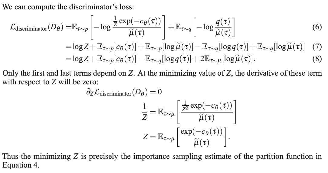
a. Discriminator의 loss를 최소화하는 Z는 partition function에 대한 importance-sampling estimator와 동일하다.
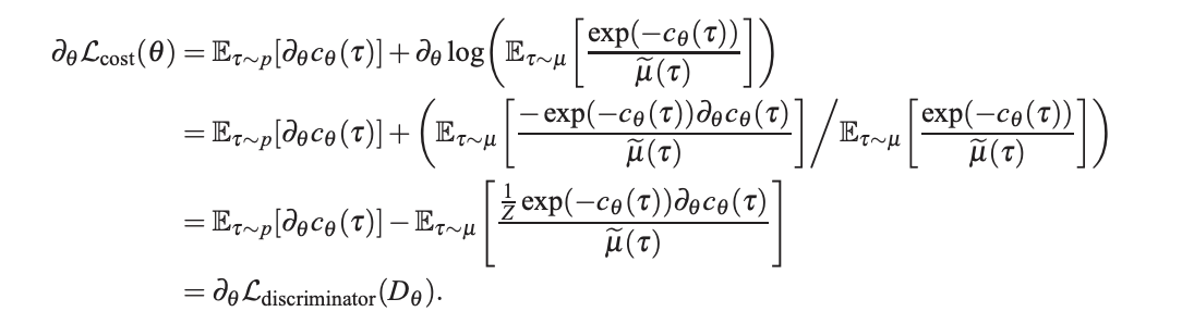
b. \(\theta\)에 대해 Discriminator’s loss와 Maximum entropy IRL’s log-likelihood objective을 미분하면 동일한 식이 나온다.
논문의 수식 (8)의 2, 4번째 term만이 \(\theta\)에 종속되어 있으므로 두 term을 \(\theta\)에 대해 미분하면 아래의 식을 얻을 수 있다.

MaxEnt IRL의 objective를 \(\theta\)에 대해 미분하면 위 공식과 동일한 결과가 유도된다!
c. Generator의 loss는 cost \(c_\theta\)와 \(q(\tau)\)의 차이며, 이는 \(L_{sampler}\)와 동일하다.
\[\begin{align*} L_{generator} (q) &= \mathbb{E}_{x \sim q} [\log (1-D(\tau))-\log D(\tau)]\\ &= \mathbb{E}_{x \sim q} [ \log \frac{q(\tau)}{\tilde{\mu}(\tau)} - \log \frac{\frac{1}{Z}\exp(-c_\theta(\tau))}{\tilde{\mu}(\tau)}]\\ &= \mathbb{E}_{x \sim q} [ \log q(\tau) + \log Z + c_\theta(\tau) ]\\ &= \mathbb{E}_{\tau \sim q} [c_\theta(\tau)] + \mathbb{E}_{\tau \sim q} [\log q(\tau)] + \log Z\\ &= L_{sampler}(q). \end{align*}\]참고로 \(Z\)는 최적화 과정에서 항상 고정되어 있는 값이므로 무시해도 무방하다.
4. GANs for training EBMs
EBM은 MaxEnt IRL에서 cost function이 energy value로 교체된 형태이므로 3과 동일한 과정으로 GAN과 EBM의 연관성을 유도해 볼 수 있다.